
To run the Price Guidance Accelerator, create a new model from the Optimization > Models menu, using the Price Guidance Model Class to instantiate the machine learning model and give it the required parameters. The model is then added to the list of models and is editable.
In this page:
New Model
-
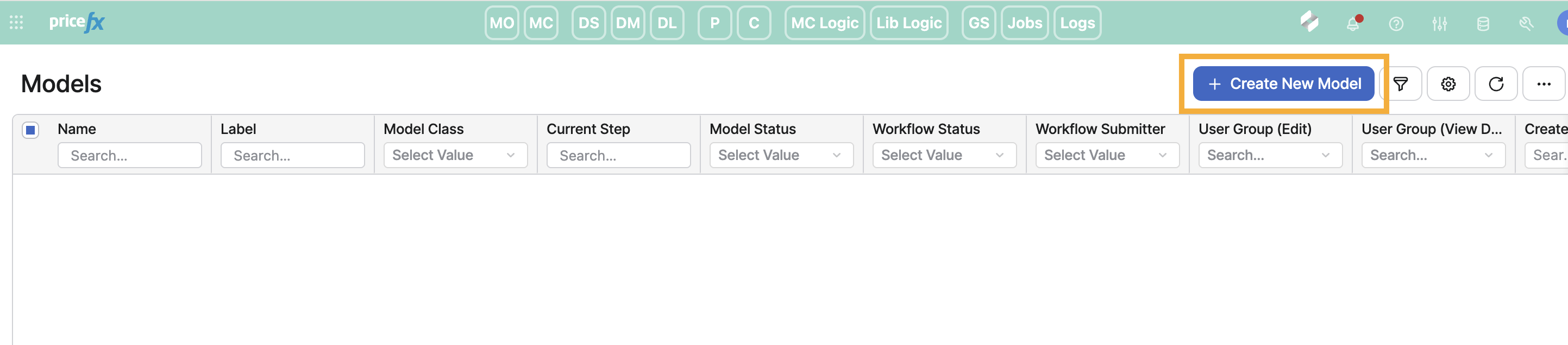
Go to Optimization > Models and add a new model.
-
Define the name of the model and choose Price Guidance as Model Class.
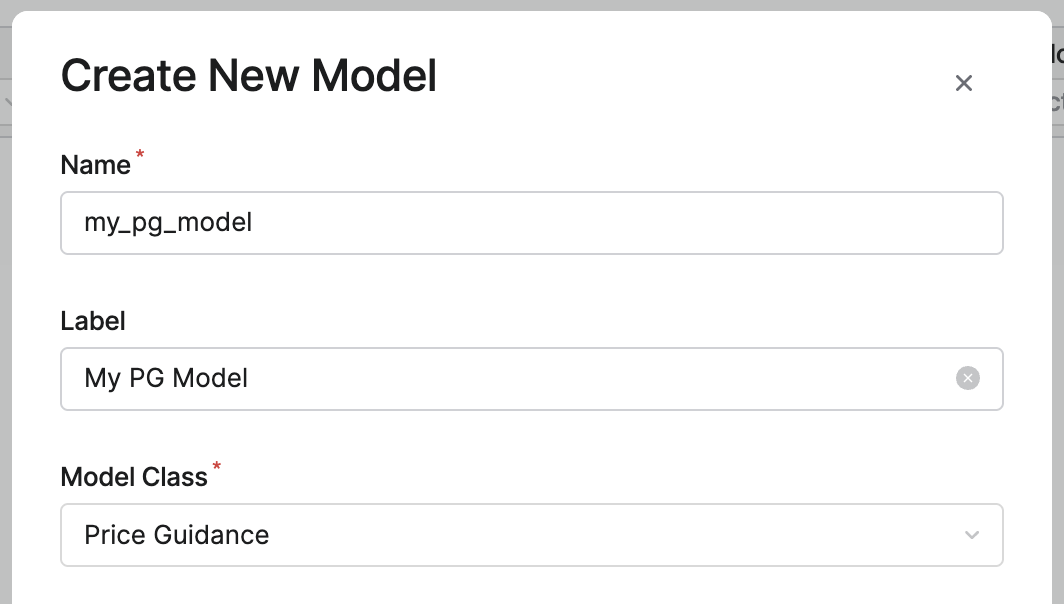
Create a Price Guidance model
The new model opens. The interface has three steps - Definition, Feature Preparation, and Results, all explained below.
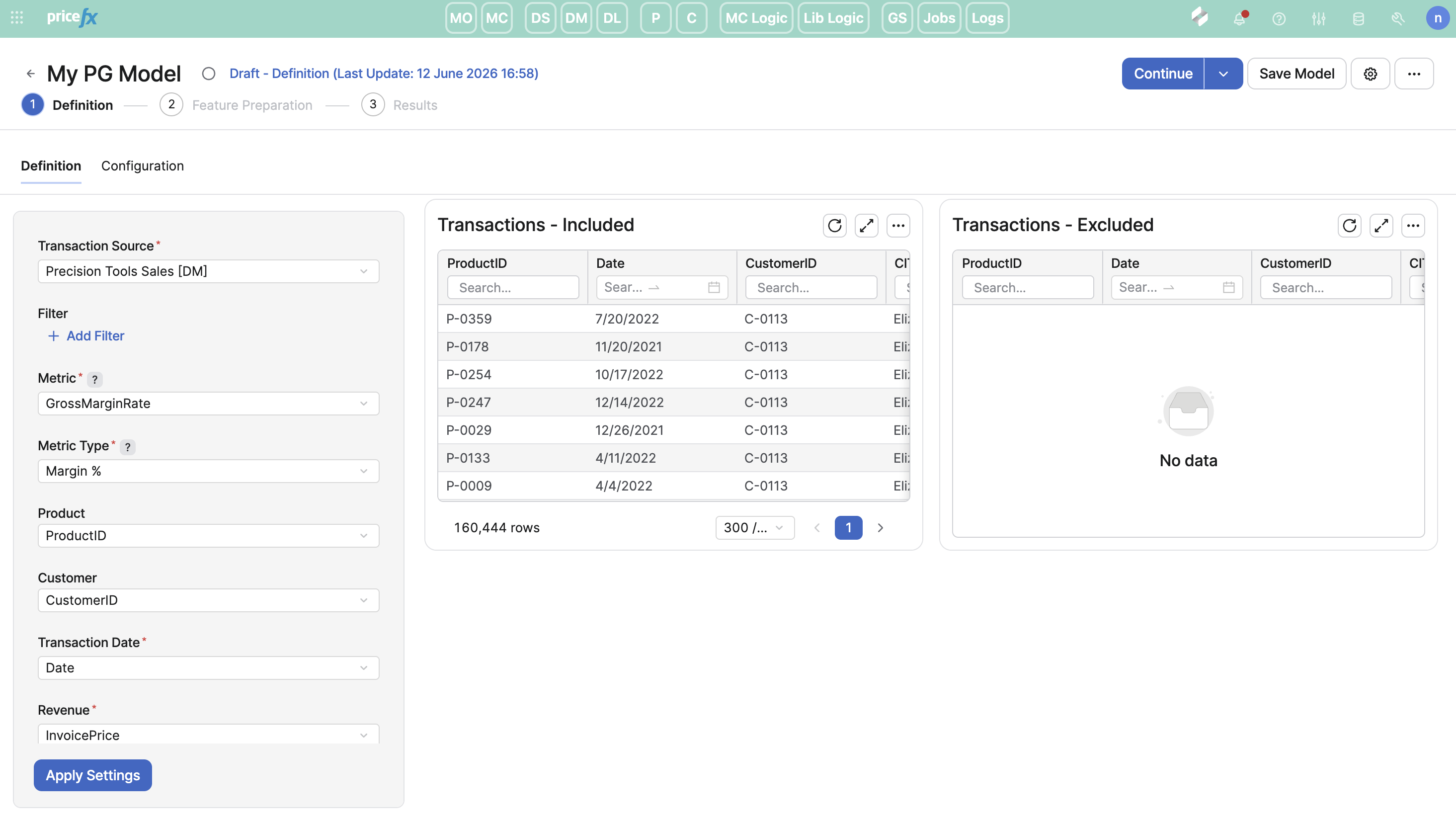
Model Steps
Definition Step
This is the first step of the model. There are two tabs: Definition and Configuration.
Definition Tab
In the Definition tab, you map the transaction source and its fields, and optionally narrow the model's scope with the Filter input. Both the source and the field mapping are pre-populated with the defaults from the accelerator's Data Mapping installation step and can be changed here without affecting those partition defaults.
There are mandatory and optional mapping fields. Their meaning is explained in Data Requirements (Optimization - Price Guidance).
-
The Metric and Metric Type together determine what the model predicts.
-
Product and Customer are optional inputs.
-
Transaction Date is used to split the data into training and test windows.
-
Revenue, Quantity, and Profit are required even when the chosen Metric is not directly derived from them - they support monetary calculations and cost-based business checks. Cost is derived as
Revenue − Profit. -
Weight is optional. When set, each transaction is weighted by this field during training, so higher-weight transactions influence the predictions more. Leave it empty to weight all transactions equally.
Weighting training rows usually improves model outputs, but the choice of weight requires business judgement. Without a weight, every transaction counts equally, so the model learns the typical price per transaction; with a quantity weight it learns the price per unit sold (the logic of a volume-weighted average price), and with a revenue weight the price per dollar of revenue. Quantity for the weight is well suited to businesses selling relatively homogeneous products at similar price levels, such as chemicals or commodities sold by the kg, square meter, volume or packaging, where one unit carries roughly the same economic importance across the catalog. It is a poor fit for heterogeneous catalogs like industrial distribution, where a screw at $0.001 sold by the thousand would dominate a piece of equipment sold one at a time for $50,000. In those cases, a revenue-based weight better reflects economic importance. Other options to not include directly the price (as revenue = price × quantity) are “revenue at list price” = list price × quantity or cost x quantity, which captures deal size without including the price. When revenue is very concentrated (e.g. a few key accounts in a B2B spare-parts business), dampen the weight with a square root or logarithm, so that a handful of large deals do not drive the model. -
Currency is the model's currency. Monetary values from a Datamart source are normalized to this currency. For a Data Source no conversion is applied and values are treated as already being in this currency.
-
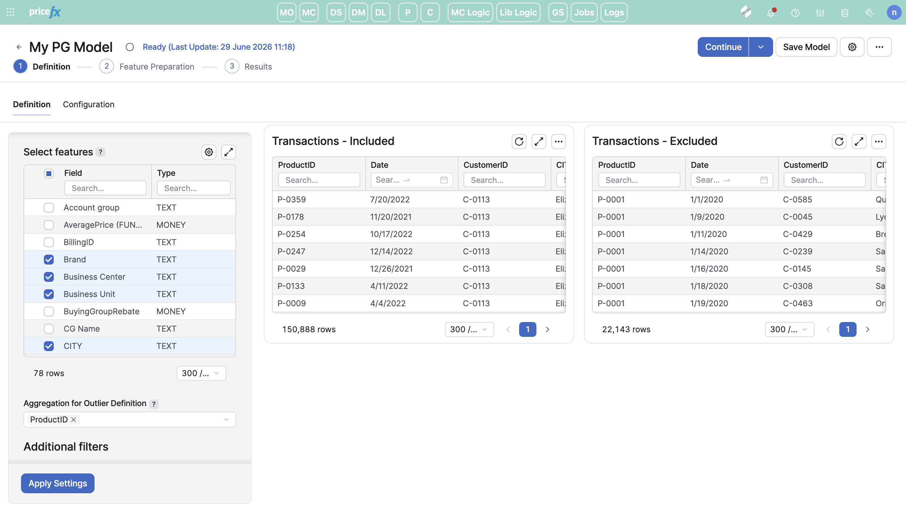
Feature Candidates is an input matrix listing the attributes that can be evaluated as model features. Select at least one candidate, but several attributes are usually required to get proper performance. This candidate set is not the final feature set - the analysis in Feature Preparation step will help you to choose which candidates to actually train on, so it is fine to be generous here.
-
Aggregation for Outlier Definition selects the fields that set the granularity of outlier detection. Outlier bounds are then computed separately within each combination of the selected field values, instead of over the whole dataset. The dropdown lists the categorical features you selected as Feature Candidates. Leave it empty to detect outliers over the entire dataset. Product ID is usually a good starting point. The fields you select here should be marked as dimensions in the source, so that they are indexed in the database.
Finally, there are three default filters that exclude transactions with negative or zero Revenue, Quantity, or derived Cost. They are useful to ensure the model runs cleanly. The boxes can be unchecked, but doing so may cause calculation failures if the underlying data contains invalid values. Transactions with an empty Metric are always excluded as well, independently of these filters.
Once you apply the settings, the right panel provides:
-
Transactions - Included - Data that will be materialized in the model and used for training.
-
Transactions - Excluded - Data that is filtered out by the source-level filter and the default negative-value filters, or because the Metric is empty.
Configuration Tab
In this tab, you set the parameters that govern the scope of the training data.
-
Outliers acceptable range - A multiplier of the interquartile range (IQR) used to determine outlier bounds on the chosen Metric. Transactions whose Metric value falls outside
[Q1 − k*IQR, Q3 + k*IQR]are excluded from training. When an Aggregation for Outlier Definition is set in the Definition tab, these bounds are computed separately within each group, otherwise they are computed over the whole dataset. Default is 1.5 (classical Tukey rule). Lower values remove more transactions. Set to 0 to skip outlier removal entirely. -
Number of days of transactions kept for the test set - A subset of the source data is reserved as a test set and is not used to train the model. It is used to check the validity of the model and avoid overfitting. The default is 30 days but can be changed. Aim for around 25% of the data in the test set, but also take care of the periodicity of the data. For instance, if your data contains a bit more than one year of transactions, it can be useful to keep exactly one year in the training set and use the start of the following year as the test set.
Once the Definition step is set up, use the Continue button at the top right to proceed to Feature Preparation.
Feature Preparation Step
This step runs a preliminary analysis to recommend which candidate features should be used for training, and collects the parameters that govern the main model's training behavior. There are two tabs: Feature Selection and Model Configuration.
Clicking Continue from the Definition step triggers the Feature Preparation calculation, which:
-
Materializes the training data and applies outlier removal based on the Outliers acceptable range set in Definition > Configuration.
-
Runs a feature-importance analysis on the candidate features picked in the Definition step.
Feature Selection Tab
This tab displays the outputs of the feature importance analysis, lets you confirm which features to actually train on, and sets whether the model predicts a single target price or a full price corridor.
Review and Check Features
In the left panel, you can find a matrix listing all candidate features. The matrix is pre-populated with the analysis's recommended subset, but you can modify this selection before triggering training. The recommended subset typically covers features whose cumulative importance accounts for the majority of the explained variance, the rest are unselected by default, to keep the training focused.
Strategy Positioning
Below the feature matrix, the Strategy input decides what the model predicts.
-
Target Only - the model predicts a single value of the target metric for each item.
-
Floor/Target/Stretch - the model predicts three values for each item, forming a price corridor: a floor, a target and a stretch price.
For the Floor/Target/Stretch strategy, you need to define the three percentiles:
-
Floor Percentile (default 10) - The percentile of comparable historical prices the floor sits at. At 10, about a tenth of comparable transactions were priced below the floor.
-
Target Percentile (default 52) - The percentile the recommended target price sits at.
-
Stretch Percentile (default 90) - The percentile the stretch price sits at. At 90, about a tenth of comparable transactions were priced above it.
These percentiles are always expressed against price, whatever the target metric is. They need to be in increasing order Floor Percentile < Target Percentile < Stretch Percentile. For Discount % metric, where a higher value means a lower price, the model inverts them internally - so a Floor Percentile of 10 still describes the low-price end of the corridor, not the low-discount end.
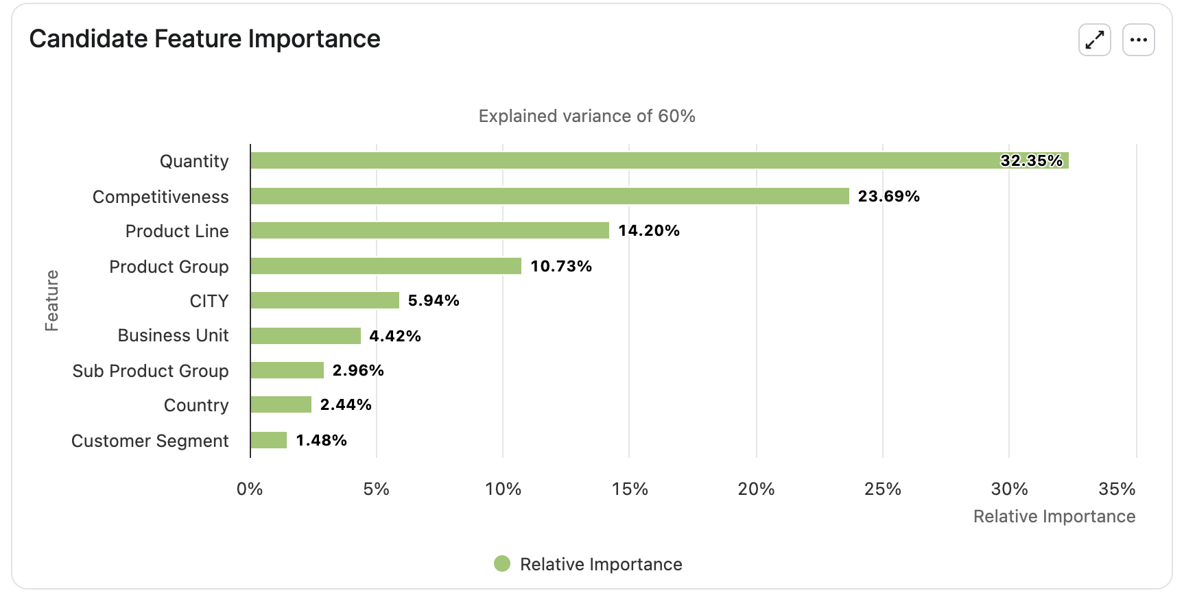
Candidate Feature Importance
A bar chart of relative importance per feature, ordered by descending importance. The subtitle shows the total explained variance - a rough indicator of how much of the target's variation the candidate features collectively explain.
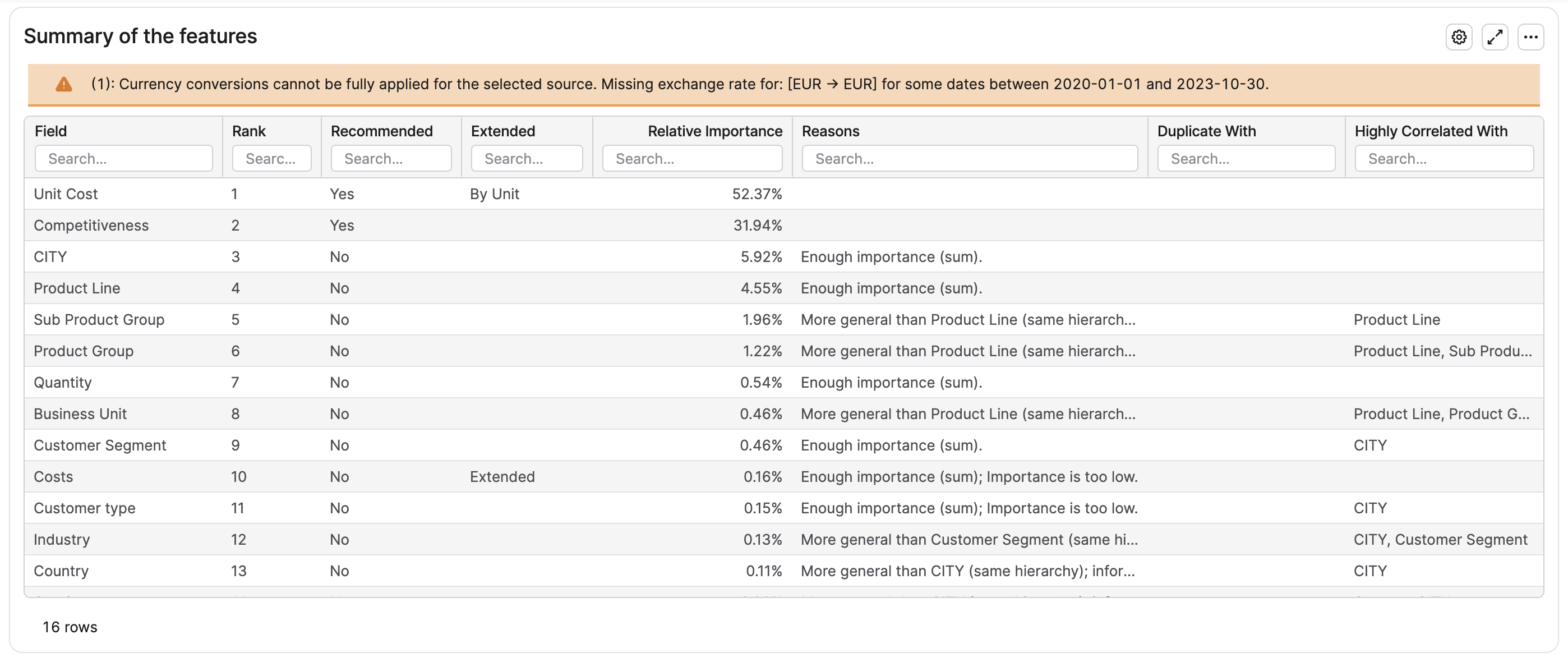
Summary of the features
A table summarizing the analysis output, ordered by descending importance. Columns:
-
Rank - order by importance.
-
Recommended - Yes/No, whether the analysis suggests including this feature.
-
Extended - for a numerical feature, whether its value already includes quantity. Extended means the value scales with quantity (for example a line revenue or an extended price), By Unit means it is a per-unit value. Empty for non-numerical (text) features.
-
Min, Max - the smallest and largest value observed for the feature.
-
Cardinality - the number of distinct values, shown for categorical features only.
-
Relative Importance - the feature's share of total importance, as a percentage.
-
Reasons - short notes explaining why a feature is or isn't recommended (e.g., low importance, duplicate of another feature, highly correlated with another feature, or another level of the same hierarchy already covers it).
-
Duplicate With - if the feature is effectively a duplicate of another candidate (identical values), the other feature is listed here.
-
Highly Correlated With - if the feature is strongly correlated with another candidate, the other feature is listed here.
Duplicates and highly correlated features are typically not recommended, keeping both adds redundancy without improving the model.
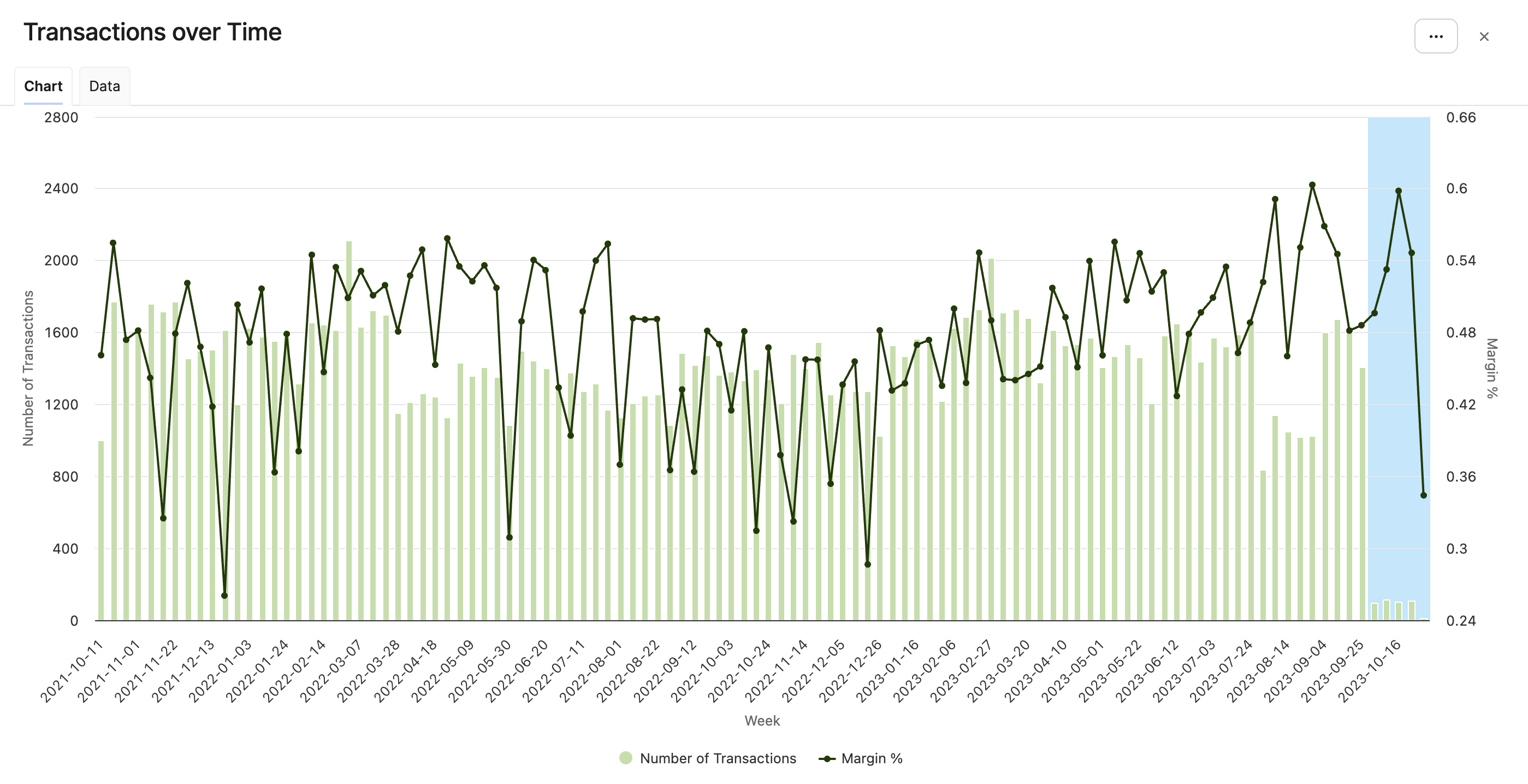
Transactions Over Time
A summary of the input transactions grouped by week, showing the periodicity of the data and how the training/test split aligns with it. Use this to check that the test window is representative - if the test set falls during an unusual period (a holiday, a price-list change, an unusually large customer), the model's measured accuracy may not reflect typical performance.
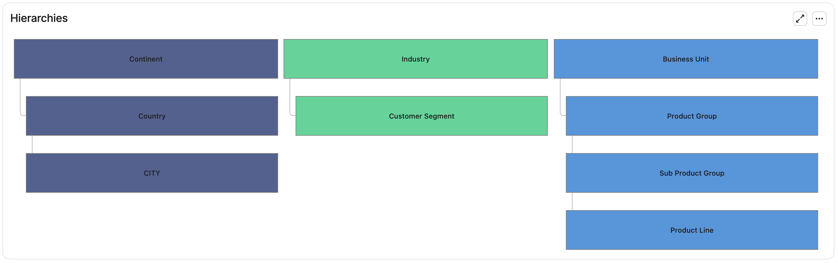
Hierarchies
This portlet visualizes features that form a hierarchical relationship in the data (for example, Product Category containing Product Subcategory containing Product Name). Including multiple levels of a hierarchy in training is usually redundant. From each connected hierarchy, the recommendation keeps only the single highest-importance feature selected.
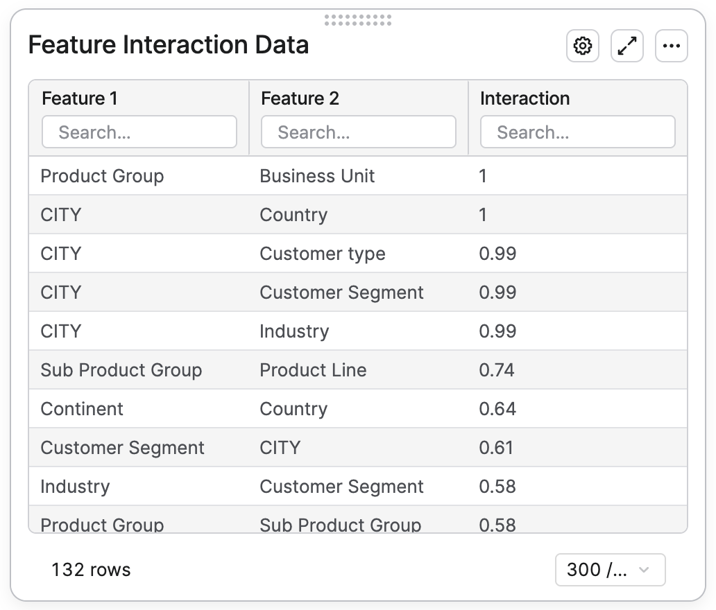
Feature Interaction Data
A table that lists every pair of features and how related they are, ordered from the most related pair at the top to the least related at the bottom. For each pair of features, Interaction is a value indicating how strongly the two features are related. Higher values mean the two features carry overlapping information and including both of them generally does not improve the model.
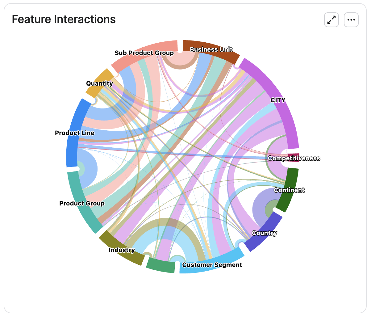
Feature Interactions
A circular chart that shows which features are most related to each other. Each feature sits around the edge of the circle, and lines connect pairs that interact - the thicker the line, the stronger the relationship. Each feature has its own color, which makes it easy to spot all the connections a single feature has.
To keep the chart readable, only the strongest interactions are shown. The busiest parts of the circle point to groups of features that say similar things about the data. Use this chart together with the Feature Interaction Data table to decide which feature to keep when several are pointing in the same direction.
Model Configuration Tab
In this tab, you set the parameters that govern the model's training behavior.
Feature Binning
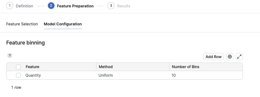
An optional input matrix that groups a numerical feature's values into bins before training, so the model learns on a single representative value per bin instead of the raw values. The matrix is empty by default. Add one row per feature you want to bin, choosing a feature, a method, and a number of bins.
In most cases, the model's automatic binning produces the most accurate result. Define manual binning only when you have a specific reason, for example a known business breakpoint or a noisy, long-tailed feature. Over-customizing bins can reduce accuracy.
Binning Quantity is usually a good practice, that removes the risk of overfitting by the model.
-
Only numerical features can be binned. The Feature dropdown lists the numerical features in scope.
-
Each binned value is mapped to its bin center, so the feature stays numerical and monotonicity constraints can still be applied to it.
-
Values outside the configured range are mapped to the nearest bin: a value below the lowest bin falls into the lowest bin, a value above the highest bin into the highest bin.
-
The available methods:
-
Uniform - bins of equal width between the feature's minimum and maximum.
-
Uniform Log - equal-width bins on a log scale, useful for values spanning several orders of magnitude.
-
Percentiles - bins that each carry an equal share of the data.
-
Long Tail - percentile-style bins that grow denser towards the extremes.
-
Custom - bin edges you define yourself, entered in the Number of Bins cell as a semicolon-separated, increasing list (for example 0;2;5;10;20;50).
-
-
Number of Bins must be a whole number of at least 2.
Model Parameters
Advanced training parameters with default values appropriate for most datasets. Adjust only if you understand the effect of the change.
|
Parameter |
Default |
Purpose |
|---|---|---|
|
Maximum Number of Training Iterations |
10 000 |
A safety cap on the number of training iterations. In practice, early stopping usually halts training well before this limit. |
|
Early Stopping |
200 |
Number of consecutive iterations without improvement on the validation set that triggers training to stop. |
|
Smoothing Iterations |
500 |
Parameter used to regularize and smooth the shape functions of continuous features during training. |
|
Number of Pairwise Adjustments |
10 |
Number of feature-pair interactions the model explicitly captures. Increasing this can lengthen training noticeably. |
|
Pairwise Smoothing Iterations |
100 |
Number of iterations used to regularize the pairwise interaction effects. |
|
Learning Rate Autoscaling |
|
Scales the learning rate to the size of the metric. |
|
Learning Rate Autoscaling Reference |
Median |
Which statistic of the training target stands for its magnitude: Median, 90th percentile or Maximum. |
|
Learning Rate Autoscaling Factor |
0.001 |
Multiplier applied to the reference statistic: |
The effective learning rate is resolved in this order: learning_rate_override from Advanced Parameters when it is set, otherwise the autoscaled value, otherwise the built-in 0.04. Whichever applies, it is never allowed below 0.0001. The resolved value is reported as Effective learning rate in Model Information portlet on Results/Metrics tab. Autoscaling is skipped when either:
-
metric is a percentage (Margin %, Discount %)
-
metric type is Other with values inside 0 to 1 interval
-
Floor/Target/Stretch strategy is selected and target normalization is on (by default)
Monotonicity Constraints
An optional input matrix to constrain selected numerical features to be monotonically increasing or decreasing in their effect on the target. Each row pairs a numerical feature with a direction.
-
Use when business logic requires the relationship to be monotonic. For example, the impact of Quantity on Unit Price should be decreasing (more units → lower unit price).
-
Enforcing monotonicity may reduce accuracy where the actual data pattern is not monotonic.

Advanced Parameters
A Parameter table holding settings that are rarely changed and are therefore kept out of the configurator. It is created the first time the Feature Preparation step calculates.
|
Parameter |
Default |
Purpose |
|---|---|---|
|
max_pairwise_combinations |
100 000 |
Upper limit on the number of value combinations a feature pair may have before it is left out of the pairwise interactions. Excluded pairs are listed in Model Information. |
|
greedy_ratio |
10.0 |
Training parameter controlling the ratio of greedy to cyclic training rounds. |
|
coverage_tolerance |
0.2 |
Floor/Target/Stretch only. How far a price level's achieved percentile may sit from the one you configured. Training of that price level fails when the gap is larger. |
|
normalize_target |
true |
Floor/Target/Stretch only. Puts the target on a common scale before the three models train. |
|
crossing_guard_epsilon |
0.0 |
Floor/Target/Stretch only. The minimum gap the evaluation keeps between the target and each bound, see the Evaluation tab. |
|
learning_rate_override |
empty |
When set, this is the learning rate and autoscaling is ignored. |
Once all the parameters are set, use the Continue button at the top right to proceed to Results - this triggers training.
Results Step
Clicking Continue from Feature Preparation triggers the model training calculation, then opens the Results step. This step has four tabs: Metrics, Feature Impact, Pairwise Impact, and Evaluation.
Throughout the Results step, chart titles and axis labels include the specific Metric Type chosen in the Definition step - for example, "Impact on recommended Margin %" or "Impact on recommended Unit Price".
Metrics Tab
This tab summarizes the trained model.
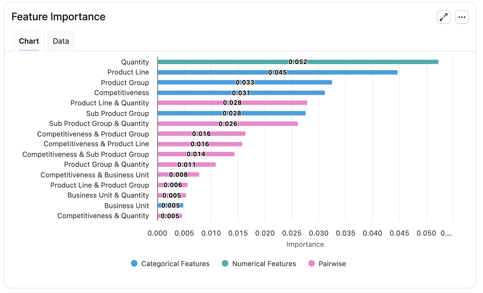
Feature Importance
A bar chart showing the importance of each feature in the trained model, ordered from most to least important. This is the importance of features as the trained model actually uses them - distinct from the Candidate Feature Importance shown during Feature Preparation, which was a preliminary estimate. Bars are colored by what they represent: Categorical Features, Numerical Features, and Pairwise, the last being a pair of features the model captured as a joint effect. With the Floor/Target/Stretch strategy the chart shows values from the target model.
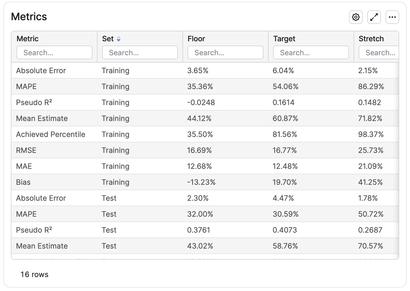
Metrics
A table comparing model performance metrics across the training set and the test set. Use this to check overfitting: if training and test values diverge significantly, the model may be overfitting and recommendations on new data will be less reliable. When a Weight field is set in the Definition tab, every metric is weighted by this weight.
-
Target Only strategy:
-
RMSE - average size of the error, in the metric's own unit, giving extra weight to large misses.
-
MAE - average size of the error, in the metric's own unit.
-
MAPE - average error as a percentage of the actual value.
-
Bias - average error relative to the average actual value. Positive means the model sits above the historical data on average, negative below.
-
R² - share of the metric's variation the model explains, 1 being a perfect fit.
-
Mean Predicted Target - average of the values the model produces.
-
-
Floor/Target/Stretch strategy:
-
RMSE - average size of the error, in the metric's own unit, giving extra weight to large misses.
-
MAE - average size of the error, in the metric's own unit.
-
MAPE - average error as a percentage of the actual value.
-
Bias - average error relative to the average actual value. Positive means the model sits above the historical data on average, negative below.
-
Pseudo R² - (Koenker and Machado's R1) the equivalent of R² for a price level, 1 being a perfect fit. This metric describes how much better the model is than recommending a single flat value for every transaction.
-
Mean Estimate - average of the values that price level produces.
-
Absolute Error - (quantile loss) average size of the error, counting misses on the wrong side of the price level more heavily than misses on the expected side.
-
Achieved Percentile - share of transactions that landed at or below the price level. Compare it with the percentile you configured in Strategy Positioning: a floor set at 10 should achieve roughly 10%.
-
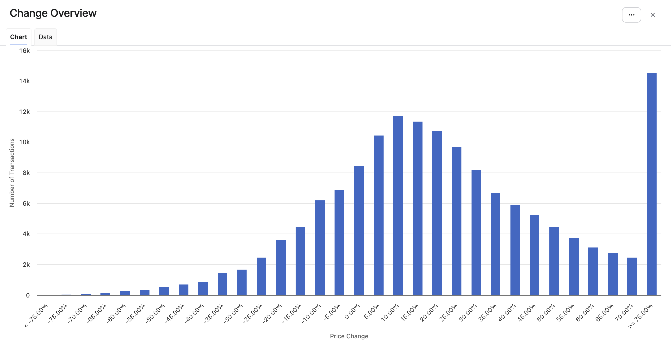
Change Overview
A histogram of the price change the recommended target implies for each transaction, relative to its historical price, so you can see how far the recommendations move the business as a whole. For metric type Other it is the relative change of the metric itself.
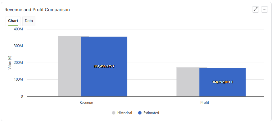
Revenue and Profit Comparison
Comparison of the historical revenue and profit of the in-scope transactions with the revenue and profit the recommended values would have produced on the same transactions. This portlet is hidden for metric type Other, because revenue and profit cannot be derived.
If there is a large gap, the recommendation is to add a weight or adjust it in the first step.
Model Information
A table of model-level facts that surface diagnostics from training, grouped in a Category column:
-
Data - training, test and calibration set sizes, the test period in days, the calibration split date, the weight field in use and how weights were normalized, and the total number of transactions excluded as outliers.
-
Features - categorical and numerical features the model trained on, any monotonicity constraints, and the excluded features that were null or constant across the training data.
-
Training - parameters the models actually trained with.
-
Reference - under the Floor/Target/Stretch strategy with at least one pairwise adjustment: the feature pairs the reference model selected for all three price levels, and its RMSE and MAE on the training and test sets.
Feature Impact Tab
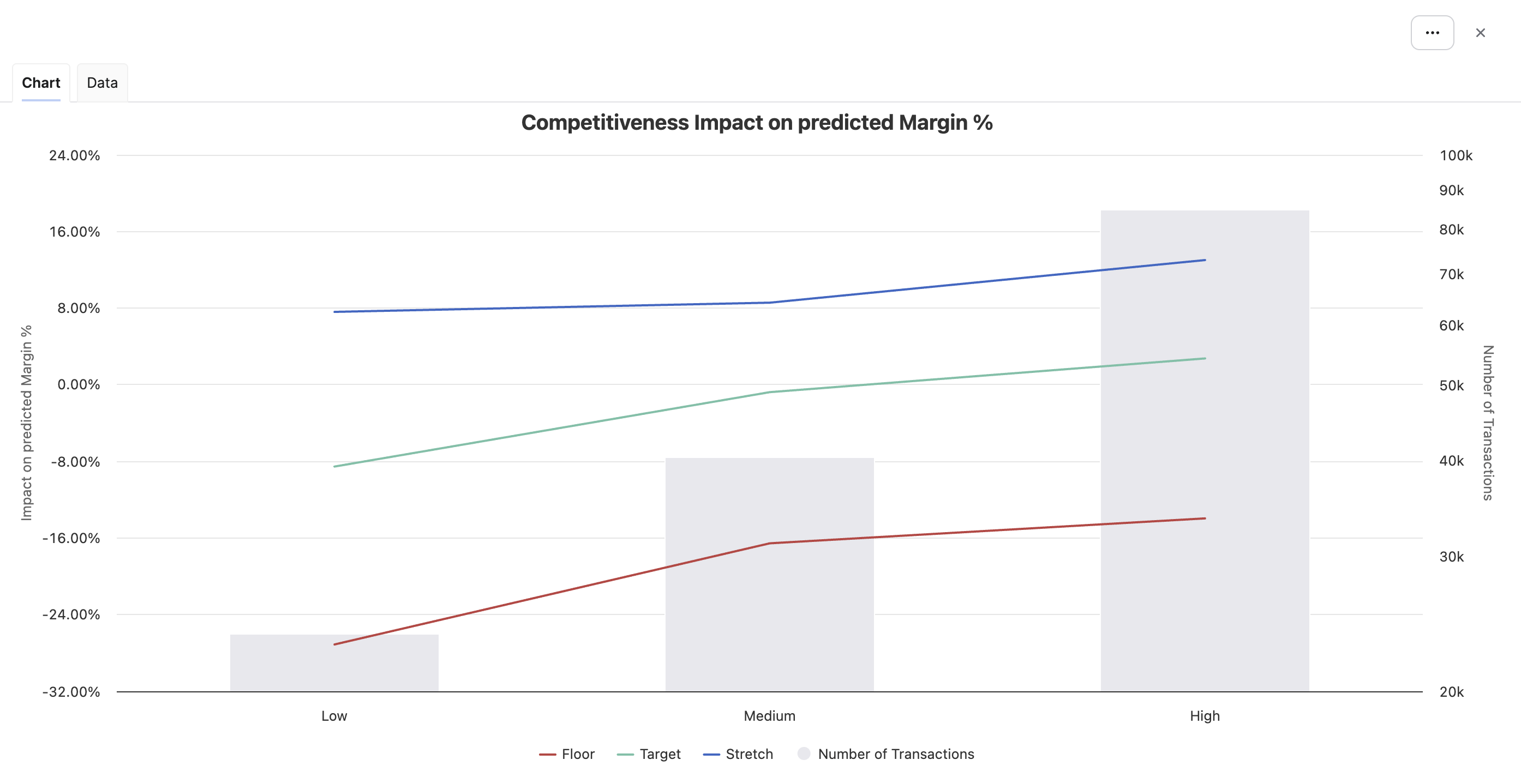
This tab shows how a chosen feature affects the prediction. In the left panel, pick a feature from the list. The dashboard then shows the feature's impact chart and, with the Floor/Target/Stretch strategy, the share of transactions across the corridor.
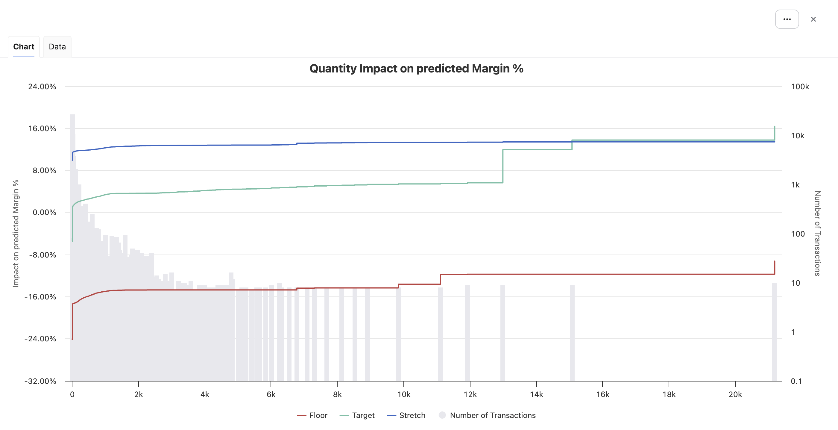
Feature Impact
A chart of the impact each value of the selected feature has on the recommended target together with number of transactions at each value.
In case of Floor/Target/Stretch strategy, the three lines are drawn against a common baseline - the target model’s Intercept. The floor and stretch lines are therefore shifted by the gap between their model's Intercept and the target model's Intercept. What you read off the chart is each price level's impact relative to the target model's baseline. Therefore, you cannot add the floor or stretch impacts across features to rebuild that price level's recommendation.
Share of Transactions relative to Floor, Target and Stretch
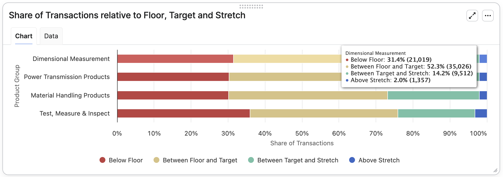
A stacked bar chart displaying how the historical transactions were split across the corridor (Below Floor, Between Floor and Target, Between Target and Stretch or Above Stretch) for each value of the selected feature. Each bar is scaled to 100%, so the bars compare composition, not volume.
Pairwise Impact Tab
This tab shows the combined impact of two features that the model captured as a pairwise interaction. In the left panel, pick Feature 1 and Feature 2. The dropdown for Feature 2 is filtered to show only valid partners for the chosen Feature 1. Not every pair of features is captured as a pairwise interaction.
With the Floor/Target/Stretch strategy, a Price Level input is present, defaulting to Target. It defines which price level is visualized in the heatmap. The tooltip always shows all three. The same pairs are offered at every price level, because all three models are trained on one shared list of feature pairs, coming from the reference model.
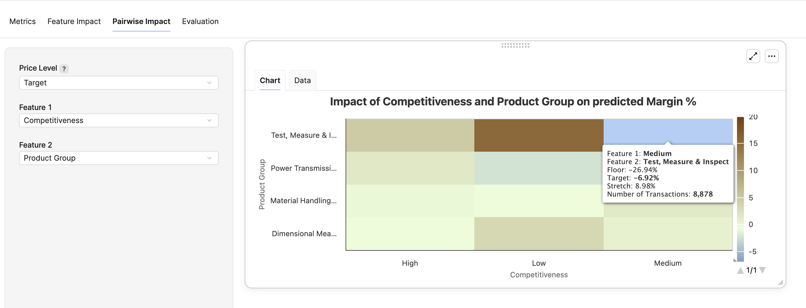
Impact heatmap
A heatmap with Feature 1 values on the X axis and Feature 2 values on the Y axis. The color shows the combined impact of the pair on the prediction:
-
Blue cells - the pair lowers the recommended target relative to what either feature contributes alone.
-
Yellow cells - no joint effect beyond what each feature contributes individually.
-
Red cells - the pair raises the recommended target.
The color scale adapts to the actual range of impact values in the heatmap. Under the Floor/Target/Stretch strategy the cells are shifted the same way as the lines in the Feature Impact chart: each price level's impact is plotted relative to the target model's Intercept, and the color, tooltip and the Data tab all show the shifted value.
Evaluation Tab
This tab recommends a value for a specific set of input values and shows what drove the recommendation. With the Floor/Target/Stretch strategy it recommends all three price levels. In the left panel, set a value for each feature in the model:
-
Categorical features - pick a value from the dropdown of values seen during training. Two special options are available:
-
Null value - explicitly sets the feature to null, matching training rows where this feature was empty. Offered only when the feature had empty values in the training data.
-
No data - the feature has a value not seen during training. The model has no contribution learned for it, so the feature adds nothing to the recommendation.
-
-
Numerical features - type the value directly.
If a feature was binned in Feature Preparation, the value you enter is mapped to its bin center before the prediction is computed. Values that fall in the same bin therefore produce the same contribution, and values outside the binned range use the nearest bin.
Overview
For Target Only strategy, displays the recommended target. For Floor/Target/Stretch strategy, displays the recommended floor, target and stretch.
The three price levels come from three separately trained models, so there is no guarantee they come out properly aligned. A crossing guard keeps them ordered: the floor and stretch are moved to maintain the required gap from the target. That gap can be configured in Advanced Parameters table as crossing_guard_epsilon parameter. You will see a notification in the portlet if a bound was moved.
Target Drivers
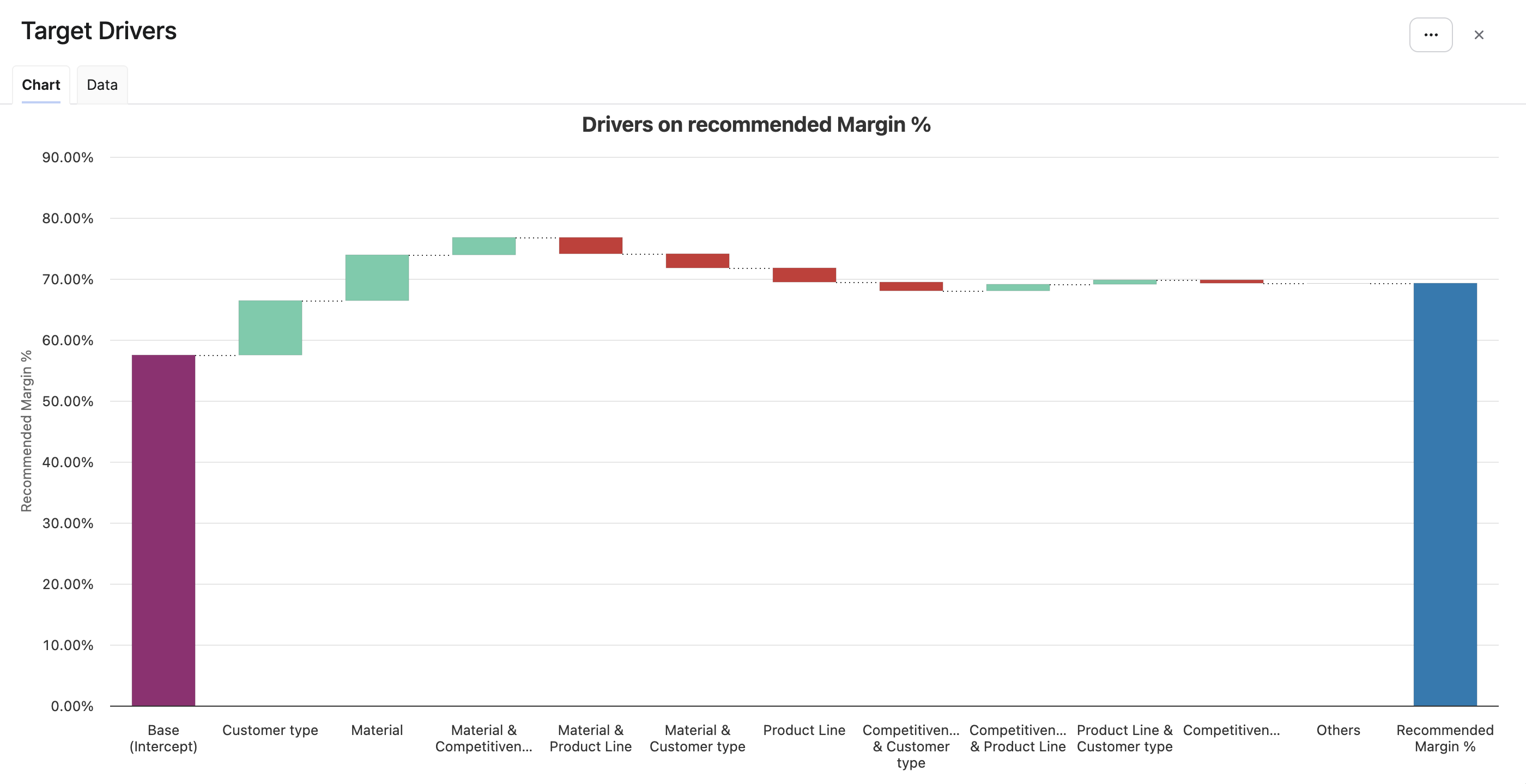
A waterfall chart showing how the prediction was built up. Each bar represents a driver
-
The first bar is the target model's baseline.
-
Each subsequent bar adds the contribution of one feature's value to the prediction. Positive contributions raise the recommended target, negative contributions lower it.
-
The final bar is the recommended target.
Drivers are listed in order of magnitude and their tooltip shows the exact contribution. With the Floor/Target/Stretch strategy, the waterfall only describes the target model.
Model Evaluation
In addition to the Evaluation tab, the model can be queried programmatically from anywhere in the Pricefx platform via the target_prediction model evaluation API. The API uses the same calculation as the Evaluation tab, so the same inputs produce the same outputs in both places.
See Technical User Reference (Optimization - Price Guidance) | Model Evaluation for the API signature, parameters, and result structure.